Introduction
This post is part 2 of a series where I discuss data loading for solving linear systems of equations. Our method extends the approach pioneerd by Gnanasekaran and Surana (2024), which I discussed in Part 1. I highly recommend that you first read Part 1, otherwise this post may not make much sense.
Here, I’ll break down the methods used in my recent article where we solved the data loading problem for the 1D Burgers’ equation - a paradigmatic nonlinear partial differential equation (PDE) relevant for fluid dynamics. Here I put solved in italics because our method applies specifically to the VQLS algorithm, which utilizes the linear combination of unitaries (LCU) theorem. It is possible that our mehtod also applies to other quantum linear system algorithms that utilize LCU, but that remains to be seen and is the subject of future work.
The goal of this writeup is as follows. Consider some (huge) matrix $\mathcal{A}\in\mathbb{R}^{N\times N}$, then we want to find $$ \begin{equation} \mathcal{A} = \sum_{l=1}^{N_s} c_l\mathcal{A}_l \end{equation} $$ where $c_l\in\mathbb{C}$ and $\mathcal{A}_l\in\mathbb{R}^{N\times N}$ are specific types of nonunitary matrices. These $\mathcal{A}_l$ are specially defined to be block encoded within unitary matrices that have efficient circuit implementations for VQLS. A key part of this method is that $N_s$ be a polylogarithmic (polylog) function of $N$, otherwise any quantum advantage is lost to data loading.
You might be wondering, isn’t it simpler to find a decomposition such that the $\mathcal{A}_l$ matrices are themselves unitary thereby saving ourselves from the block encoding step? The answer is yes, that is the ideal approach. However, there are instances when this sort of decomposition is not possible with an $N_s$ that is polylog. In those instances, our block encoding method is simply an alternative for data loading and requires only a single qubit more of overhead.
Transforming from Nonlinear to Linear
Before we discuss data loading, we first need to setup the problem. Consider the generic second order nonlinear ordinary differential equation (ODE)
$$\begin{equation}\tag{1}\label{eqn:IVP} \frac{\partial \vec{f}}{\partial t} = F_1 \vec{f} + F_2\vec{f}^{\otimes 2} \end{equation}$$
where $\vec{f}(t) = \bigl( f_1(t),\dots,f_N(t) \bigr)^T\in\mathbb{R}^N$ and $F_k\in\mathbb{R}^{N\times N^k}$ for $k\in\{1,2\}$. The Burgers’ equation can be written in the above form, but for now we will work with the generalized form.
Next, we implement the following on eq. \eqref{eqn:IVP}:
- Carleman linearization from Liu et al. (2021) – transforms our finite nonlinear ODE into an infinite linear ODE,
- Truncation of the infinite ODE to order $\alpha$ – forms a finite linear ODE,
- Temporal discretization using backward Euler with $n_t$ time steps of size $\Delta t$ – transforms the finite linear ODE into a finite linear system of equations.
These methods transform eq. \eqref{eqn:IVP} into a linear system of equations of the form $L\vec{Y}=\vec{B} $ where $L\in\mathbb{C}^{n_t\Delta\times n_t\Delta}$, $\Delta=\sum_{j=1}^\alpha N^j$, and $\vec{Y},\vec{B}\in\mathbb{C}^{n_t\Delta}$. A solution to this linear system provides an approximate solution to our original nonlinear ODE. Note that, while the accuracy of the problem improves with increasing $\alpha$, the size of the linear system unfortunately scales exponentially with $\alpha$. This tension means that choosing the appropriate $\alpha$ is critical.
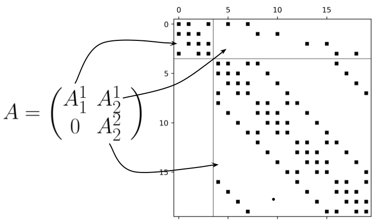
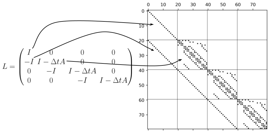
So, what is this matrix $L$ and how does it relate to eq. \eqref{eqn:IVP}? Let’s pick it apart piece by piece to see. By definition $$L = \begin{pmatrix} \tag{2} \label{eqn:L} I & 0 & \dots & 0 \\ -I & I-\Delta t A & \dots & 0 \\ \vdots & \ddots & \ddots & \vdots \\ 0 & \dots & -I & I-\Delta t A \end{pmatrix}, $$ where each block in $L$ evolves the system forward by $\Delta t$ with $n_t$ total blocks. To continue to pick $L$ apart, we break open the $A$ matrices defined by $$ \begin{equation} \tag{3} \label{eqn:A} A = \begin{pmatrix} A_1^1 & A_2^1 & 0 & … & 0 \\ 0 & A_2^2 & A_3^2 & … & 0 \\ \vdots & \dots & \ddots & \ddots & \ddots \\ 0 & \dots & \dots & A_{\alpha-1}^{\alpha-1} & A_\alpha^{\alpha-1} \\ 0 & \dots & \dots & 0 & A_\alpha^\alpha \end{pmatrix} \end{equation} $$ where we can see that the size of $A$ depends upon the truncation order $\alpha$. By inspection of $A$, we identify two types of block matrices: $A_j^j$ and $A_{j+1}^j$ defined by $$ \begin{equation} A_j^j = \sum_{l=0}^{j-1} I_{n_x}^{\otimes l} \otimes F_1 \otimes I_{n_x}^{\otimes j-l-1}, \quad A_{j+1}^j = \sum_{l=0}^{j-1} I_{n_x}^{\otimes l} \otimes F_2 \otimes I_{n_x}^{\otimes j-l-1} . \end{equation} $$ You can think of the $A_j^j$ and $A_{j+1}^j$ blocks as implementing the dynamics contained in the $F_1$ and $F_2$ matrices respectively. The example below should help you get a better feeling for the structure of this kind of matrix.
Example 1
Consider the 1D spatially discretized Burgers' equation $$\begin{equation} \frac{\partial u_j}{\partial t} = \underbrace{\frac{\nu}{\Delta x^2}(u_{j+1} - 2u_j + u_{j-1})}_{F_1\vec{u}} - \underbrace{\frac{u_j}{2\Delta x}(u_{j+1}-u_{j-1})}_{F_2\vec{u}^{\otimes 2}} \end{equation} $$ where $u_j(t)=(u_1(t),\dots,u_{n_x}(t))^T$, $\nu$ is the diffusion coefficient, and $\Delta x$ is the grid spacing. This can be rewriten into the form of eq. \eqref{eqn:IVP} where the $F_1$ and $F_2$ terms are shown in the underbraces.Let's consider the example where $n_x=4$ and $\alpha=2$. The $A$ matrix defined from eq. \eqref{eqn:A} takes the form in the figure below.
Now let's see how these matrices fit into the $L$ matrix from eq. \eqref{eqn:L} when $n_t=4$.
So, now that we have gained some intuition about the structure of $L$, how would you go about decomposing it into a linear combination of unitaries with, importantly, a number of terms ($N_s$) that is polylog?
One of the challenges in doing this is that even though we know that $L$ is composed of these $A$ blocks, the differing sizes of the $A_j^j$ and $A_{j+1}^j$ terms makes it difficult to separate them out. But what if each $A_j^j$ and $A_{j+1}^j$ were the same size? Then, it becomes much easier to pick $A$, and thereby $L$, apart. This is exactly what I introduce in the next section.
Carleman Embedding
To circumvent the issue of each of the $A_j^j$ and $A_{j+1}^j$ blocks being differently sized, we’ll use zero-padding to force their sizes to be equal. Define $$ \begin{equation} A_j^{(e),j} = \begin{pmatrix} A_j^j & 0 \\ 0 & 0 \end{pmatrix}, \quad A_{j+1}^{(e),j} = \begin{pmatrix} A_{j+1}^j & 0 \\ 0 & 0 \end{pmatrix}, \end{equation} $$ where the superscript $(e)$ stands for “embed” and the $0$ blocks are appropriately sized. Whereas $A_j^j$ and $A_{j+1}^j$ are sized $N^j \times N^j$ and $N^j \times N^{j+1}$ respectively, their embedded analogs $A_j^{(e),j}$ and $A_{j+1}^{(e),j}$ are sized $N^\alpha \times N^\alpha$ for all $j$. We then use these blocks to form a matrix analogous to \eqref{eqn:A} given by $$ \begin{equation} \tag{4} \label{eqn:Ae} A^{(e)} = \begin{pmatrix} A_1^{(e),1} & A_2^{(e),1} & 0 & … & 0 \\ 0 & A_2^{(e),2} & A_3^{(e),2} & … & 0 \\ \vdots & \dots & \ddots & \ddots & \ddots \\ 0 & \dots & \dots & A_{\alpha-1}^{(e),\alpha-1} & A_\alpha^{(e),\alpha-1} \\ 0 & \dots & \dots & 0 & A_\alpha^{(e),\alpha} \end{pmatrix} . \end{equation} $$
Given this new definition of $A^{(e)}$, we can then define an analogous linear system of equations of the form $L^{(e)} \vec{Y}^{(e)} = \vec{B}^{(e)}$ where $$ L^{(e)} = \begin{pmatrix} \tag{5} \label{eqn:Le} I & 0 & \dots & 0 \\ -I & I-\Delta t A^{(e)} & \dots & 0 \\ \vdots & \ddots & \ddots & \vdots \\ 0 & \dots & -I & I-\Delta t A^{(e)} \end{pmatrix} . $$ Even though this linear system is substantially larger than the previous version, we are using size as a resource enabling us to easily “pick” out each of the $A_j^j$ and $A_{j+1}^j$ blocks with limited overhead. This is demonstrated in the following example.
Example 2
Consider again the setup from Example 1 with $n_x=4$, $n_t=4$, and $\alpha=2$. Then the structure of the $A^{(e)}$ matrix from eq. \eqref{eqn:Ae} looks a lot like the $A$ matrix, but with judicious zero-padding.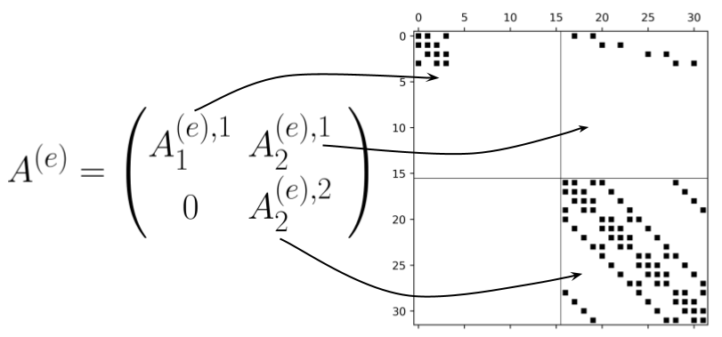
The decomposition of $L^{(e)}$ from eq. \eqref{eqn:Le} is also made easier since it is given by $$ \begin{equation} L^{(e)} = (\rho_4^{\otimes 2} - \rho_0\otimes\rho_0) \otimes A^{(e)} + (\rho_4^{\otimes 2} - \rho_4\otimes\rho_2 - \rho_2\otimes\rho_1) \otimes\rho_4^{\otimes 5}. \end{equation} $$
So, by inserting $A^{(e)}$ into $L^{(e)}$ we simply need to find decompositions for $A_1^{(e),1}$, $A_2^{(e),1}$, and $A_2^{(e),2}$, which is a much easier problem than the original one of needing to find a decomposition for $L$ from eq. \eqref{eqn:L}.
This demonstrates the key advantage of using this Carleman embedding (zero-padding) method. That being said, our job is not over since we must now decompose each of the $A_j^{(e),j}$ and $A_{j+1}^{(e),j}$ terms. But, importantly, we have reduced the problem from a daunting one to one that is more manageable. In Part 3 of this series, I will show how to fully decompose the matrix $L^{(e)}$ introduced here into explicit circuits to be run with the VQLS method.
Questions or comments? ReubenDemi [at] gmail [dot] com
References
[1] A. Gnanasekaran and A. Surana, “Efficient Variational Quantum Linear Solver for Structured Sparse Matrices,” 2024 IEEE International Conference on Quantum Computing and Engineering (QCE), Montreal, QC, Canada, 2024, pp. 199-210, doi: 10.1109/QCE60285.2024.00033
[2] Demirdjian, Reuben, Thomas Hogancamp, and Daniel Gunlycke. “An Efficient Decomposition of the Carleman Linearized Burgers’ Equation.” arXiv preprint arXiv:2505.00285 (2025).
[3] Bravo-Prieto, Carlos, et al. “Variational quantum linear solver.” Quantum 7 (2023): 1188.
[4] Liu, Jin-Peng, et al. “Efficient quantum algorithm for dissipative nonlinear differential equations.” Proceedings of the National Academy of Sciences 118.35 (2021): e2026805118.